[EN]Grid-based clustering method - Wave cluster wavelet clustering

✨The easy-to-run .ipynb note book is now available on Github: BaiHLiu/WaveCluster

Overview of lattice clustering methods

Introduction

A clustering algorithm is an unsupervised classification algorithm. There are many algorithms, including division-based clustering algorithms (e.g., kmeans), hierarchical clustering algorithms (e.g., BIRCH), density-based clustering algorithms (e.g., DBScan), lattice-based clustering algorithms, and so on.

Based on the division and hierarchical clustering methods are unable to discover non-convex shape clusters, the real effective algorithm to discover arbitrary shape clusters is density-based algorithms, but the density-based algorithms are generally higher time complexity, between 1996 and 2000, research data mining scholars proposed a large number of lattice-based clustering algorithms, lattice methods can effectively reduce the computational complexity of the algorithm, and the same sensitive to density parameters.

So, A one sentence summary of the core idea of several clustering methods:

• Based on division: points within classes are close enough and points between classes are far enough. We keep replacing the clustering centre until it is stable, which is the final result.
• Based on density: first discover the points with higher density, and then gradually connect the similar high density points together, and then form clusters.
• Grid-based: Divide the data space into a grid, map the data into grid cells (cells) according to certain rules, and then calculate the density of each cell. According to a pre-set threshold to determine whether each grid cell is a high-density cell, by the adjacent high-density cells to form a class.

Basic steps

Grid-based clustering methods use a multi-resolution grid data structure that quantifies the object space into a finite number of cells that form a grid structure on which all clustering operations are performed.

Before that, let’s go through the concept of Resolution.

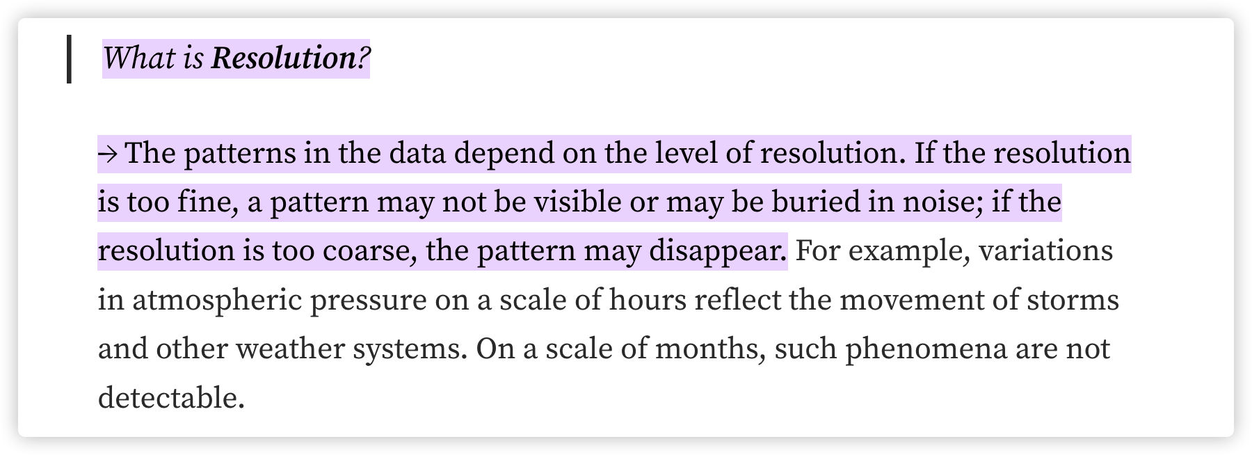
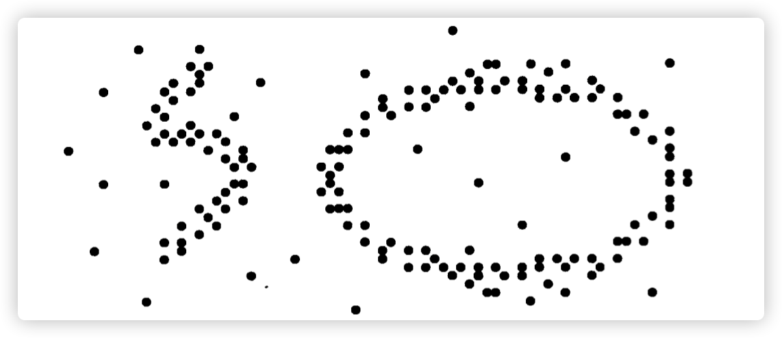
And the two following figures show how resolution affect.

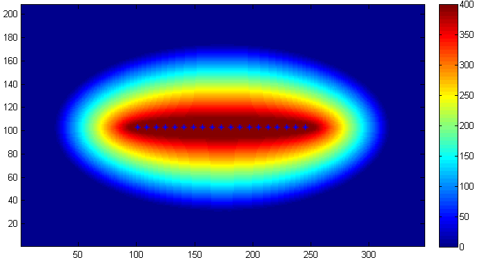
Overall, the different resolutions determine whether to get more generalised or more detailed information.

Different algorithms have different methods of grid delineation and handle the grid data structure differently, but the core steps are the same:

1. delimit the grid
2. use statistical information about the data within the grid cells to compressively represent the data
3. determine high density grid cells based on this information
4. identify connected high-density grid cells as clusters

Some examples of grid clustering methods

Statistical Information Grid (STING) algorithm

**Core Idea

First we start by dividing some levels, actually each level here corresponds to a resolution of the sample.

Each high-level cell is divided into multiple cells in the next level, and each cell calculates its statistical information, which is pre-calculated and stored as statistical parameters.

Using such a structure, it is easy to perform a query, starting from the top to the bottom, calculating the confidence interval of the query at each cell based on the cell’s statistical information, finding the largest cell, then going to the next layer, and so on until we get to the bottom layer. The advantage of this is that we don’t have to calculate all the samples, the algorithm discards irrelevant samples at each level, less and less computation is needed, and then the speed will be fast.

Commonly used statistics parameters

• count The number of objects in the grid.
• mean The mean of all values in the grid.
• stdev The standard deviation of the attribute values in the grid.
• min Minimum value of the attribute in the grid
• max The maximum value of a property in the grid.
• distribution The type of distribution that the attribute values in the grid conform to. (eg: normal distribution, uniform distribution)

STING algorithm query steps: (already calculated in advance parameters))

• (1) Start from one level
• (2) For each cell of this level, we calculate the value of the attribute associated with the query.
• (3) From the computed attribute values and with the constraints, we mark each cell as relevant or not wanting to be relevant. (Irrelevant cells are no longer considered and the next lower level of processing checks only the remaining relevant cells)
• (4) If this level is the bottom level, then go to (6), otherwise go to (5)
• (5) we move from the hierarchy to the next level, in accordance with step (2) to proceed
• (6) The query is satisfied, go to step 8, otherwise (7)
• (7) Restore the data to the relevant cell for further processing to get satisfactory results, go to step (8)
• (8) Stop.

If the granularity tends to 0 (i.e. towards very bottom data), the clustering result tends to the DBSCAN clustering result.

Relation to density-based clustering: if the granularity of the grid tends to 0 (i.e. towards very bottom data, i.e. very high resolution), the clustering result tends to the DBSCAN clustering result.

Advantages:

• Grid-based computations are query-independent, as the statistics stored in each cell provide aggregated information about the data in the cell, independent of the query.

• The grid structure facilitates incremental updating and parallel processing.

  Incremental updating: the algorithm discards irrelevant samples at each level and does not need to update them all.

  Parallel processing: each grid has little connection with each other, and the parameters are calculated separately.

• Efficiency: STING scans the database once to compute the statistics of the cells, so the time complexity of generating clusters is O(n), and after the hierarchy is built, the query processing time is )O(g),where g is the number of bottom grid cells, which is usually much less than n.

Disadvantages:

• There is no diagonal dividing line, cluster boundaries are only horizontal and vertical.
• Due to the multi-resolution mechanism, the quality of clustering depends on the granularity of the bottom layer of the grid structure. If the granularity of the lowest level is very fine, the cost of processing increases significantly. However, if the granularity is too coarse, the clustering quality is difficult to be guaranteed.

CLIQUE algorithm (subspace clustering algorithm)

The CLIQUE algorithm is a lattice-based spatial clustering algorithm, but it also combines very well with density-based clustering algorithms, and thus is capable of discovering arbitrarily shaped clusters, as well as handling larger multidimensional data like the lattice-based algorithms.

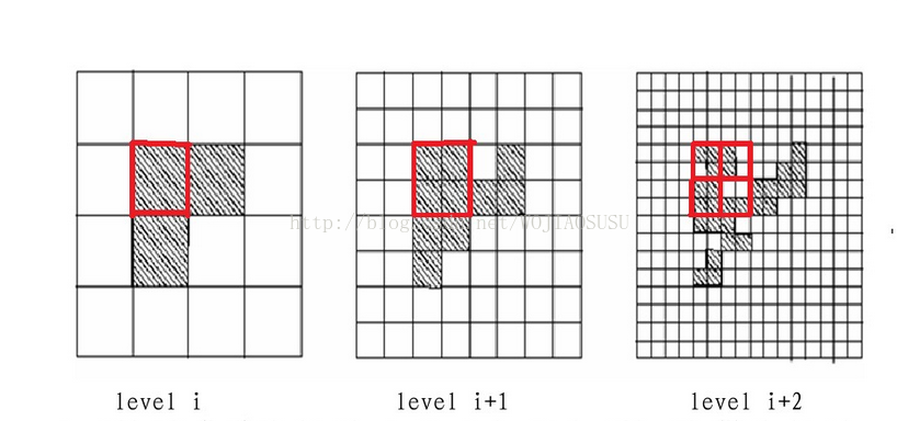
Core idea: dense grid merging

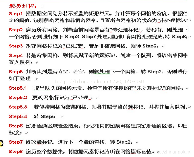
All grids are first scanned. When the first dense grid is found, expansion is started with that grid. The principle of expansion is that if a grid is neighbouring a grid in a known dense region and is itself dense, that grid is added to that dense region until no more such grids are found. The scanning of grids is then continued and the process is repeated until all grids have been traversed.

Algorithm flow

The summary is: first determine if a mesh is a dense mesh, and if it is, then iterate over its neighbouring meshes to see if they are dense. If it is, then iterate over its neighbouring meshes to see if they are dense, and if they are, then they belong to the same cluster.

Advantages:

• Although the number of potential grid cells can be high, only need to create grids for non-empty cells.
• The time complexity of assigning each object to a cell and calculating the density of each cell is O(m) and the whole clustering process is very efficient.

Disadvantages:

• Like most density-based clustering algorithms, lattice-based clustering relies heavily on the choice of the density threshold.

  (Too high, clusters may be lost. Too low, clusters that should be separated may be merged)

• As the dimensionality increases, the number of grid cells increases rapidly (exponentially). I.e., for higher dimensional data, clustering is less effective.

Wave Cluster

Wave Cluster, known as wavelet clustering, is a fast grid-based clustering method commonly used for multi-dimensional large-scale data containing a large number of outliers.

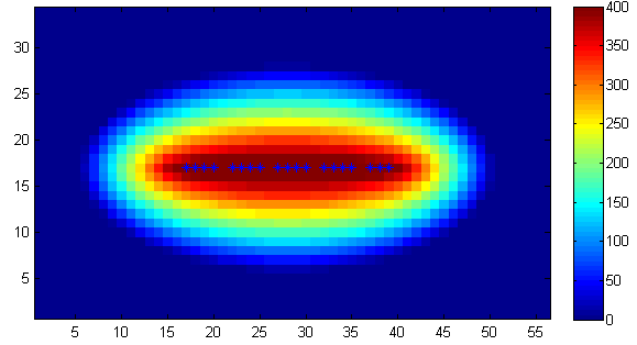
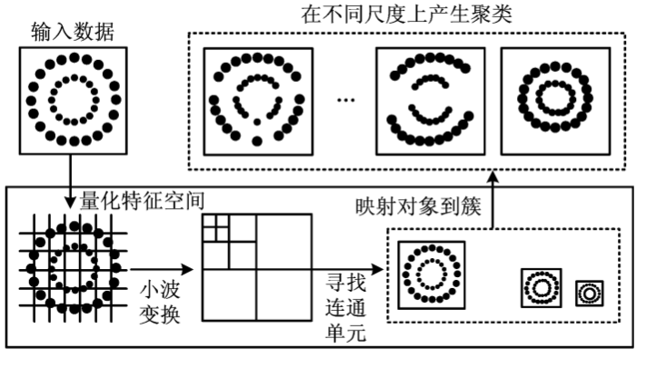
The principal idea

is to treat multidimensional data as a multidimensional signal. It first divides the data space into a grid structure, and then transforms the data space into a frequency domain space by wavelet transform, in which the natural clustering property of the data is revealed by making a convolution with a kernel function. Due to the multi-resolution nature of the wavelet transform, information on details can be obtained at high resolution, and information on contours can be obtained at low resolution.

Preliminaries: discrete wavelet transform (DWT)

The Discrete Wavelet Transform is a discretisation of the scale and translation of the underlying wavelet. In image processing, binary wavelets are often used as the wavelet transform function, i.e., they are divided using integer powers of 2.

Wavelet Transform Concepts

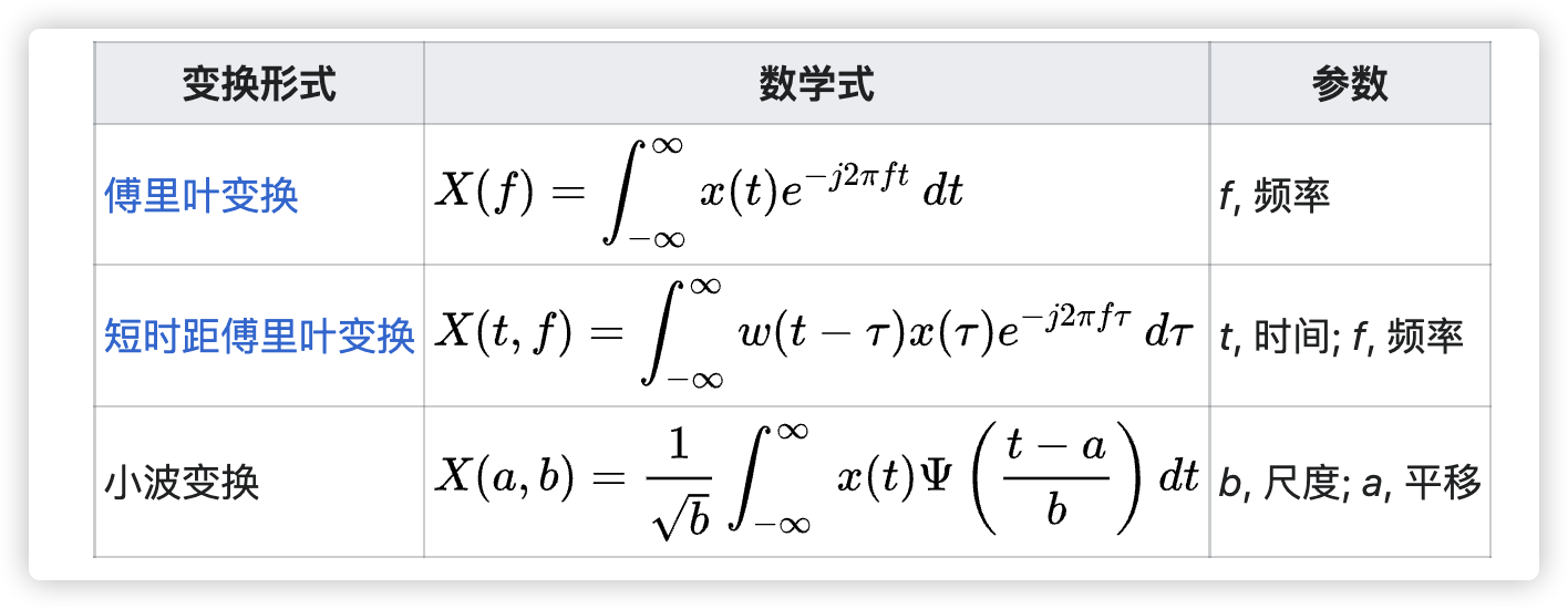
Let’s first review the Fourier transform.

The Fourier transform is a linear integral transform that is used to transform a function (called a ‘signal’ in applications) between the time and frequency domains. The effect is to decompose a function into a sum of sinusoidal functions with different characteristics.

Simply put: all waves can be represented as a superposition of many sinusoids. Example: fitting a square wave.

The wavelet transform analyses both time and frequency just like the Fourier transform, but the wavelet transform has better time resolution at high frequencies and better frequency resolution at low frequencies.

Input and output are continuous functions called Continuous Wavelet Transform; output and output are discrete values called Discrete Wavelet Transform, discrete wavelet transform is often used in signal coding.

Image Compression*

For many signals, their low-frequency components are often embedded in the basic characteristics of the signal, while the high-frequency signals only give information about the details of the signal, such as information about the edge contours of an image signal.

DWT example

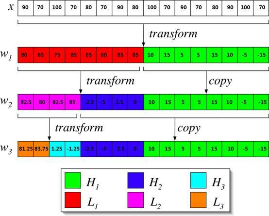
x0,x1,x2,x3=90,70,100,70

In order to achieve compression effect, take (x0+x1)/2 (x0-x1)/2 to represent the new x0,x1

90,70 is represented as 80,10 80 is the average (frequency) and 10 is the number of small fluctuations (amplitude).

Similarly 100,70 is represented as 85,15

80 and 85 are localised averages, reflecting frequencies, called Low-Pass.

10 and 15 are small fluctuations in amplitude, called High Frequency Part (High-Pass)

That is, 90,70,100,70 after a wavelet transform, can be expressed as 80,85,10,15, the low-frequency part of the front (L), the high-frequency part of the back (H)

Perform three wavelet transforms on the following sequence:

Basic principle

The core idea of the WaveCluster algorithm is that after dividing the data space into a grid, the wavelet transform is performed on this grid data structure, and then the high-density regions in the transformed space are identified as clusters. Based on the assumption that the number of data points is greater than the number of grid cells (N ≥ K), the time complexity of WaveCluster is O(N), where N is the number of data points in the dataset and K is the number of grid cells in the grid.

The WaveCluster algorithm requires two parameters:

• Size of the grid - to determine the spatial grid division
• Density threshold - the number of objects in the grid is greater than or equal to this threshold indicating that the grid is dense

**Algorithm Flow

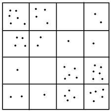
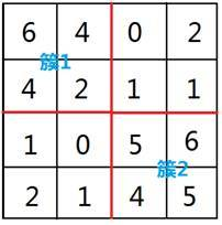
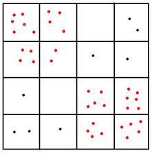
1. discretise the original space into a mesh space and place the original data into the corresponding cells to form a new feature space

   

2. perform wavelet transform on the feature space, i.e. compress the original data with wavelet transform

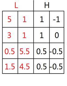
   1. Perform wavelet transform on each row to get

      

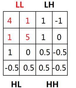
   2. Then wavelet transform is applied to each column of **, and we get

   

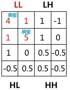
3. Find the lattice in the wavelet transformed LL space with density greater than a threshold (3 in this case) and mark it as dense

   

4. for the grids with connected densities as a cluster, label them with the cluster number of the cluster they are in

   

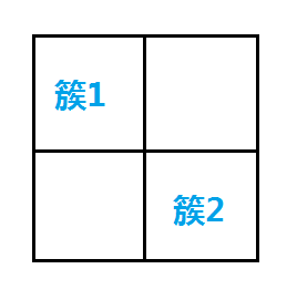
5. Create a mapping table of the cells before and after the conversion, and map the cluster labels to the original map.

   

6. Map the original data to the respective clusters

   

Effect of parameter tuning on results

From the above analysis, the parameters that can be tuned for wavelet clustering are:

• Sparsity of the grid (called scale, scale or level in some articles)
• Density threshold

Results evaluation analysis

nmi (normalised mutual information)

Information gain IG(Y|X): measures how much uncertainty about Y is reduced by knowing X

Mutual Information I(X;Y): measures the information shared by X and Y. Measures how much the uncertainty about the other is reduced by knowing one of these two

Both are numerically identical.

Theoretically, the larger the value of mutual information, the better, but there is no upper bound on the range of its values. In order to better compare different clustering results, the concept of standardised mutual information is proposed, which normalises the value of mutual information** to between 0 and 1**, so that comparisons can be made between different data sets. The closer the value of normalised mutual information is to 1, the better the clustering results.

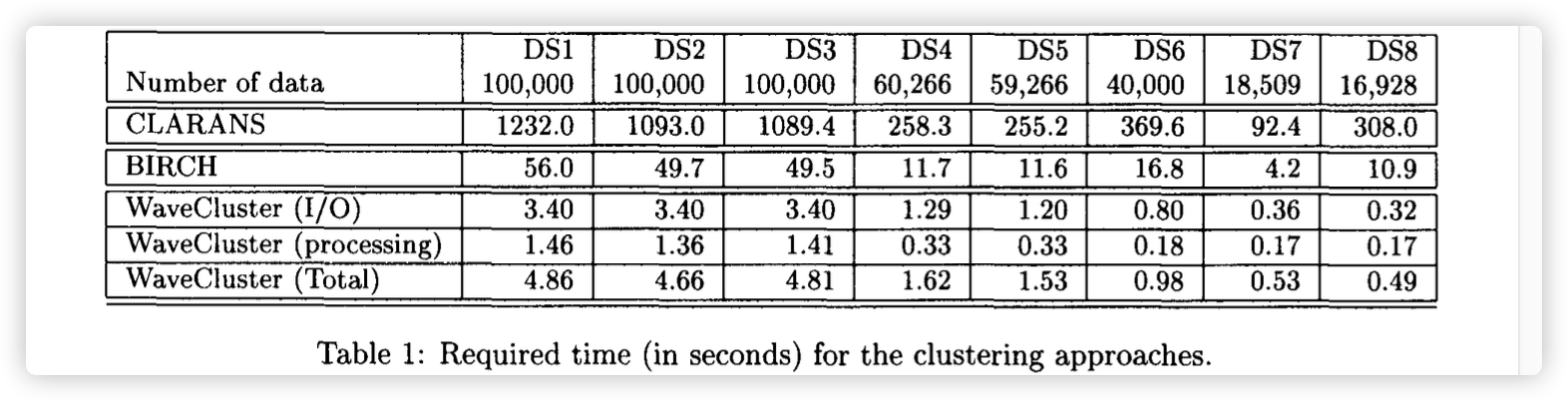
The metrics given on the original paper:

Main advantages

• Algorithmic complexity of O(n) for low dimensionality, suitable for huge datasets
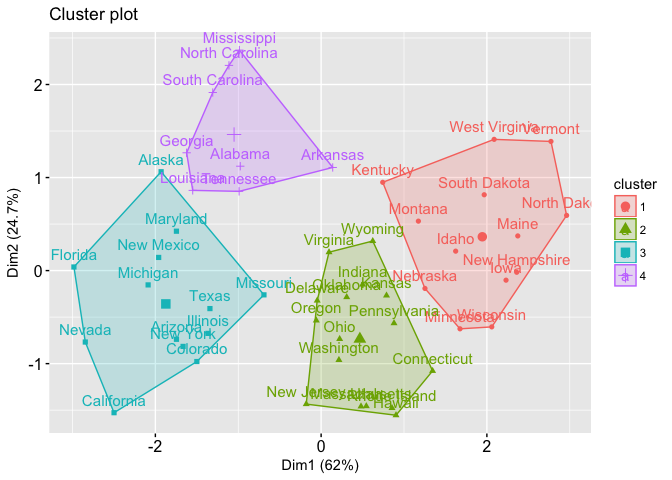
• Recognises arbitrary shapes
• Multi-resolution, can find clusters of arbitrary complex structures according to user-specified scale
• Good noise immunity

Disadvantages

• Parameter sensitive, clustering results are very dependent on the choice of density threshold and grid size

  If the threshold is too high, clusters may be lost; if the threshold is too low, those that should be separated may be combined

• Grid cells grow exponentially with increasing dimensionality

  i.e. clustering results are often poor and time consuming for high dimensional data.

Improved algorithm

Dual grid correction algorithm

`[1]刘晓波,邵伟芹,张明明,左红艳.基于双网格校正小波聚类的转子故障诊断[J].计算机集成制造系统,2017,23(09):1883-1890.DOI:10.13196/j.cims.2017.09.007.

Problem Causes:

• There is no proper criterion for the optimal quantisation of the grid, thus there is no pre-destination for this approach, only a blind search until a result is found.
• At the same time, uniform grid quantisation of the space with one size yields grid cells consisting of volumes of equal size, but since the distribution of spatial data objects is often uneven**, uniform quantisation with only one size will mask the fact that the data objects are unevenly distributed within the grid cells, thus reducing the accuracy of the clustering.

Solution: Apply two dimensions to quantise the space and apply correction algorithm to correct the clustering results to improve the clustering accuracy.

EXPERIENCE: **reduces the impact of grid partitioning and grid density thresholds on clustering quality; changes the grid partitioning scale from blind to heuristic. **

Parallel wavelet algorithm

Yıldırım A A, Özdoğan C. Parallel WaveCluster: A linear scaling parallel clustering algorithm implementation with application to very large datasets[J]. Journal of Parallel and Distributed Computing, 2011, 71(7): 955-962.

Extended clustering speed and scale under parallel processing conditions by using wavelet transforms at different scale levels.

Improved wavelet clustering algorithm based on peaked lattices

[1]龙超奇,蒋瑜,谢雨.基于峰值网格改进的小波聚类算法[J].计算机应用,2021,41(04):1122-1127.

Problem cause: the wavelet clustering algorithm does not make good use of the grid values after wavelet transform, and only segments them by density threshold.

Solution: Improve the judgement method of connectivity region and introduce the concept of ‘peak grid’.

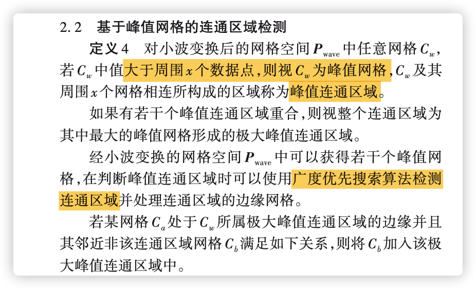
Under the same low grid scale, this method uses the grid of high-density regions to faster search for connected regions according to the cluster centre, and also can partition different cluster classes under lower grid scales, resulting in better clustering results.

Summary

The grid clustering algorithm is a clustering algorithm that is also sensitive to the density parameter, which can effectively reduce the computational complexity of the algorithm. The grid-based spatial representation of the data makes it multi-resolution, but at the same time the effect is also quite sensitive to the grid scale.

Wave Cluster first grid structure to summarise the data, and then uses a wavelet transform to transform the original feature space and find dense regions in the transformed space. The clustering of wavelet transform is very fast with O(n) computational complexity.

Application Scenarios

paper